Structural DNA helical parameters from MD trajectory tutorial using BioExcel Building Blocks (biobb)

Based on the NAFlex server and in particular in its Nucleic Acids Analysis section.

---

This tutorial aims to illustrate the process of extracting structural and dynamical properties from a DNA MD trajectory helical parameters, step by step, using the BioExcel Building Blocks library (biobb). The particular example used is the Drew Dickerson Dodecamer sequence -CGCGAATTCGCG- (PDB code 1BNA, https://doi.org/10.2210/pdb1BNA/pdb). The trajectory used is a 500ns-long MD simulation taken from the BigNASim database (NAFlex_DDD_II entry).

---

Settings

Biobb modules used

• biobb_dna: Tools to analyse DNA structures and MD trajectories.

Auxiliary libraries used

• jupyter: Free software, open standards, and web services for interactive computing across all programming languages.

• matplotlib: Comprehensive library for creating static, animated, and interactive visualizations in Python.

Conda Installation & Launch

git clone https://github.com/bioexcel/biobb_wf_dna_helparms.git
cd biobb_wf_dna_helparms
conda env create -f conda_env/environment.yml
conda activate biobb_dna_helparms_tutorial
jupyter-notebook biobb_wf_dna_helparms/notebooks/biobb_dna_helparms_tutorial.ipynb

---

Pipeline steps

1. Input Parameters

2. Running Curves+ and Canal

3. Average Helical Parameters

   1. Base Pair Step (Inter Base Pair) Parameters

   2. Base Pair (Intra Base Pair) Parameters

   3. Axis Parameters

   4. Grooves

   5. Backbone Torsions

4. Time Series Helical Parameters

5. Stiffness

6. Bimodality

7. Correlations

   1. Sequence Correlations: Intra-base pairs

   2. Sequence Correlations: Inter-base pair steps

   3. Helical Parameter Correlations: Intra-base pairs

   4. Helical Parameter Correlations: Inter-base pair steps

   5. Neighboring steps Correlations: Intra-base pairs

   6. Neighboring steps Correlations: Inter-base pair steps

8. Questions & Comments

---

---

# Auxiliary libraries

import os
import shutil
import glob
from pathlib import Path, PurePath
import zipfile
import matplotlib.image as mpimg
import matplotlib.pyplot as plt
import pandas as pd
from IPython.display import Image
import ipywidgets

Input parameters

Input parameters needed:

• seq: Sequence of the DNA structure (e.g. CGCGAATTCGCG)

• seq_comp: Complementary sequence of the given DNA structure (e.g. CGCGAATTCGCG)

• traj: Trajectory for a 500ns Drew Dickerson Dodecamer MD simulation (taken from BigNASim)

• top: Associated topology for the MD trajectory

# Input parameters
seq = "CGCGAATTCGCG"
seq_comp = "CGCGAATTCGCG"

traj = "TRAJ/structure.stripped.nc"
top = "TRAJ/structure.stripped.top"

# Auxiliary lists
grooves = ('majd','majw','mind','minw')
axis_base_pairs = ('inclin','tip','xdisp','ydisp')
base_pair = ('shear','stretch','stagger','buckle','propel','opening')
base_pair_step = ('rise','roll','twist','shift','slide','tilt')
backbone_torsions = ('alphaC', 'alphaW', 'betaC', 'betaW', 'gammaC', 'gammaW', 'deltaC', 'deltaW', \
'epsilC', 'epsilW', 'zetaC', 'zetaW', 'chiC', 'chiW', 'phaseC', 'phaseW')

Running Curves+ and Canal

---

Curves+ program and its associated Canal tool allow us to extract helical parameters from a DNA MD simulation.

Curves+ is a nucleic acid conformational analysis program which provides both helical and backbone parameters, including a curvilinear axis and parameters relating the position of the bases to this axis. It additionally provides a full analysis of groove widths and depths. Curves+ can also be used to analyse molecular dynamics trajectories. With the help of the accompanying program Canal, it is possible to produce a variety of graphical output including parameter variations along a given structure and time series or histograms of parameter variations during dynamics.

Conformational analysis of nucleic acids revisited: Curves+
R. Lavery, M. Moakher, J. H. Maddocks, D. Petkeviciute, K. Zakrzewska
Nucleic Acids Research, Volume 37, Issue 17, 1 September 2009, Pages 5917–5929
https://doi.org/10.1093/nar/gkp608

CURVES+ web server for analyzing and visualizing the helical, backbone and groove parameters of nucleic acid structure.
C. Blanchet, M. Pasi, K. Zakrzewska, R. Lavery
Nucleic Acids Research, Volume 39, Issue suppl_2, 1 July 2011, Pages W68–W73
https://doi.org/10.1093/nar/gkr316 http://curvesplus.bsc.es

---

Building Blocks used:

• curves from biobb_dna.curvesplus.biobb_curves

• canal from biobb_dna.curvesplus.biobb_canal

---

The extraction of helical parameters is then done in two steps:

• Step 1: Curves+: Reading input MD trajectory and analysing helical parameters.

• Step 2: Canal: Taking Curves+ output and generating time series and/or histograms of parameter variations during dynamics.

---

Step 1: Curves+

Curves+ program needs a trajectory and its associated topology, and a couple of ranges, informing about the numeration of the two DNA strands: s1range and s2range.

Important: Depending on the operating system used, the cell below can return an error about a missing .curvesplus folder. In this case, please copy the .curvesplus folder provided in the repository and copy it into the /path/to/anaconda3/envs/biobb_dna_helparms_tutorial folder in your computer.

from biobb_dna.curvesplus.biobb_curves import biobb_curves

curves_out_lis = "curves.out.lis"
curves_out_cda = "curves.out.cda"

prop = {
    's1range' : '1:12',
    's2range' : '24:13'
}

biobb_curves(
    input_struc_path=traj,
    input_top_path=top,
    output_lis_path=curves_out_lis,
    output_cda_path=curves_out_cda,
    properties=prop
)

Step 2: Canal

Canal program needs the output of the previous Curves+ execution, and is able to produce time series (series property) and histograms (histo property) for the parameter variations during dynamics.

from biobb_dna.curvesplus.biobb_canal import biobb_canal

canal_out = "canal.out.zip"

prop = {
    'series' : True,
    'histo' : True
}

biobb_canal(
    input_cda_file=curves_out_cda,
    input_lis_file=curves_out_lis,
    output_zip_path=canal_out,
    properties=prop
)

Extracting Canal results in a temporary folder

canal_dir = "canal_out"

if Path(canal_dir).exists(): shutil.rmtree(canal_dir) 
os.mkdir(canal_dir)

with zipfile.ZipFile(canal_out, 'r') as zip_ref:
    zip_ref.extractall(canal_dir)

Extracting Average Helical Parameters

Average helical parameter values can be computed from the output of Curves+/Canal execution.

The helical parameters can be divided in 5 main blocks:

• Helical Base Pair Step (Inter-Base Pair) Helical Parameters

• Helical Base Pair (Intra-Base Pair) Helical Parameters

• Axis Base Pair

• Grooves

• Backbone Torsions

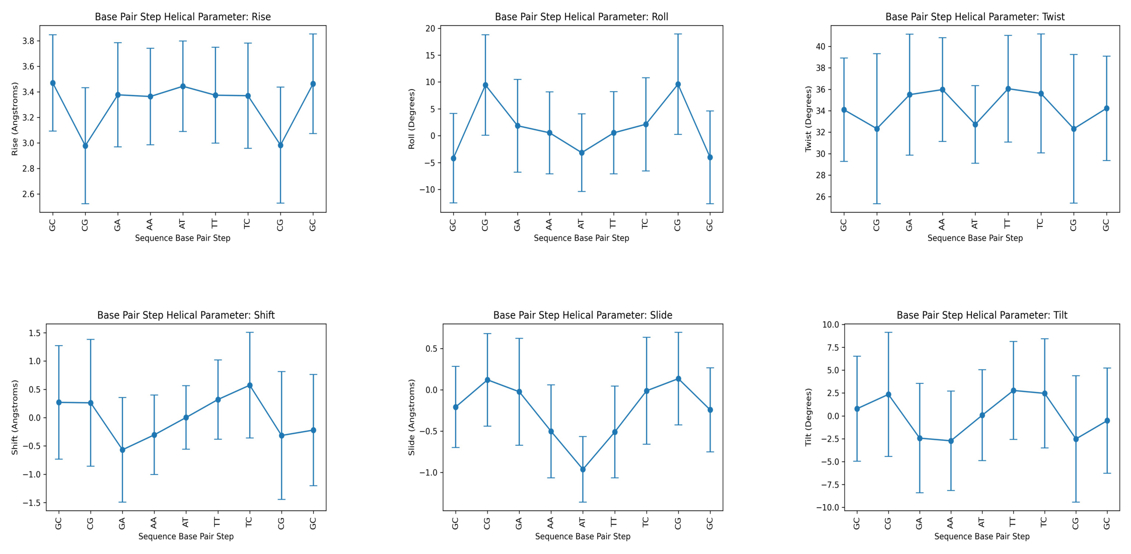
Helical Base Pair Step (Inter Base Pair) Parameters

Translational (Shift, Slide, Rise) and rotational (Tilt, Roll, Twist) parameters related to a dinucleotide Inter-Base Pair (Base Pair Step).

• Shift: Translation around the X-axis.

• Slide: Translation around the Y-axis.

• Rise: Translation around the Z-axis.

• Tilt: Rotation around the X-axis.

• Roll: Rotation around the Y-axis.

• Twist: Rotation around the Z-axis.

---

---

Building Block used:

• dna_averages from biobb_dna.dna.dna_averages

---

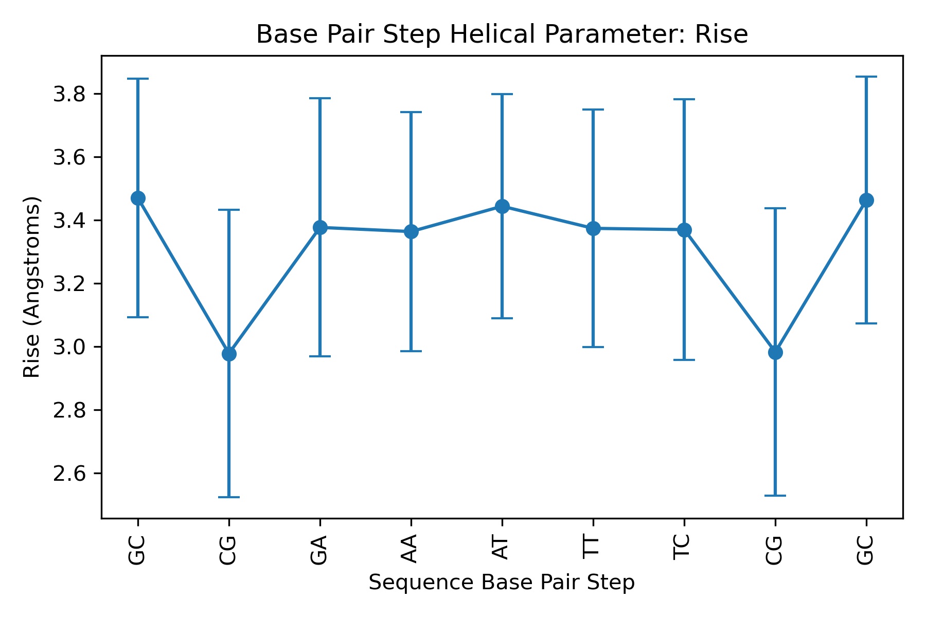
Extracting a particular Helical Parameter: Rise

from biobb_dna.dna.dna_averages import dna_averages

helpar = 'rise'

input_file_path = "canal_out/canal_output" + "_" + helpar + ".ser"
output_averages_csv_path= helpar+'.averages.csv'
output_averages_jpg_path= helpar+'.averages.jpg'

prop = {
    'helpar_name': helpar,
    'sequence': seq
}

dna_averages(
    input_ser_path=input_file_path,
    output_csv_path=output_averages_csv_path,
    output_jpg_path=output_averages_jpg_path,
    properties=prop)

Showing the calculated average values for Rise helical parameter

output_averages_csv_path= helpar+'.averages.csv'
df = pd.read_csv(output_averages_csv_path)
df

	Base Pair Step	mean	std
0	GC	3.470550	0.377972
1	CG	2.978038	0.454661
2	GA	3.377096	0.408705
3	AA	3.363942	0.378155
4	AT	3.444138	0.355242
5	TT	3.374110	0.376290
6	TC	3.370114	0.411934
7	CG	2.982740	0.454215
8	GC	3.464096	0.390428

Plotting the average values for Rise helical parameter

Image(filename=output_averages_jpg_path,width = 600)

Computing average values from all base-pair step parameters

from biobb_dna.dna.dna_averages import dna_averages

for helpar in base_pair_step:

    input_file_path = "canal_out/canal_output" + "_" + helpar + ".ser"
    output_averages_csv_path= helpar+'.averages.csv'
    output_averages_jpg_path= helpar+'.averages.jpg'

    prop = {
        'helpar_name': helpar,
        'sequence': seq
    }

    dna_averages(
        input_ser_path=input_file_path,
        output_csv_path=output_averages_csv_path,
        output_jpg_path=output_averages_jpg_path,
        properties=prop)

Showing the calculated average values for all base-pair step helical parameters

for helpar in base_pair_step:
    output_averages_csv_path= helpar+'.averages.csv'
    df = pd.read_csv(output_averages_csv_path)
    print("Helical Parameter: " + helpar)
    print(df)
    print("---------\n")

Helical Parameter: rise
  Base Pair Step      mean       std
0             GC  3.470550  0.377972
1             CG  2.978038  0.454661
2             GA  3.377096  0.408705
3             AA  3.363942  0.378155
4             AT  3.444138  0.355242
5             TT  3.374110  0.376290
6             TC  3.370114  0.411934
7             CG  2.982740  0.454215
8             GC  3.464096  0.390428
---------

Helical Parameter: roll
  Base Pair Step      mean       std
0             GC -4.192414  8.331507
1             CG  9.446606  9.363419
2             GA  1.852456  8.644153
3             AA  0.536582  7.624018
4             AT -3.163010  7.237972
5             TT  0.534468  7.656334
6             TC  2.127450  8.682155
7             CG  9.585186  9.365877
8             GC -4.021720  8.647046
---------

Helical Parameter: twist
  Base Pair Step       mean       std
0             GC  34.088546  4.816438
1             CG  32.326028  6.989191
2             GA  35.500510  5.637390
3             AA  35.972860  4.838027
4             AT  32.721506  3.618198
5             TT  36.053014  4.974014
6             TC  35.610722  5.545855
7             CG  32.319386  6.922376
8             GC  34.228190  4.863295
---------

Helical Parameter: shift
  Base Pair Step      mean       std
0             GC  0.269898  1.002226
1             CG  0.261994  1.120109
2             GA -0.568252  0.924852
3             AA -0.303916  0.701930
4             AT  0.003008  0.560834
5             TT  0.320328  0.700562
6             TC  0.573412  0.934916
7             CG -0.315024  1.130856
8             GC -0.220348  0.982379
---------

Helical Parameter: slide
  Base Pair Step      mean       std
0             GC -0.207536  0.492641
1             CG  0.121372  0.560931
2             GA -0.023312  0.648352
3             AA -0.502846  0.563088
4             AT -0.963374  0.396783
5             TT -0.510682  0.556494
6             TC -0.011398  0.648248
7             CG  0.135720  0.561489
8             GC -0.242346  0.509866
---------

Helical Parameter: tilt
  Base Pair Step      mean       std
0             GC  0.788582  5.737113
1             CG  2.352174  6.790473
2             GA -2.433898  5.987960
3             AA -2.723502  5.435644
4             AT  0.072902  4.969859
5             TT  2.780530  5.351470
6             TC  2.466076  5.965965
7             CG -2.520270  6.909690
8             GC -0.519486  5.749269
---------

Plotting the average values for all base-pair step helical parameters

images = []
for helpar in base_pair_step:
    images.append(helpar + '.averages.jpg')

f, axarr = plt.subplots(2, 3, figsize=(40, 20))

for i, image in enumerate(images):
    y = i%3
    x = int(i/3)

    img = mpimg.imread(image)

    axarr[x,y].imshow(img, aspect='auto')
    axarr[x,y].axis('off')

plt.show()

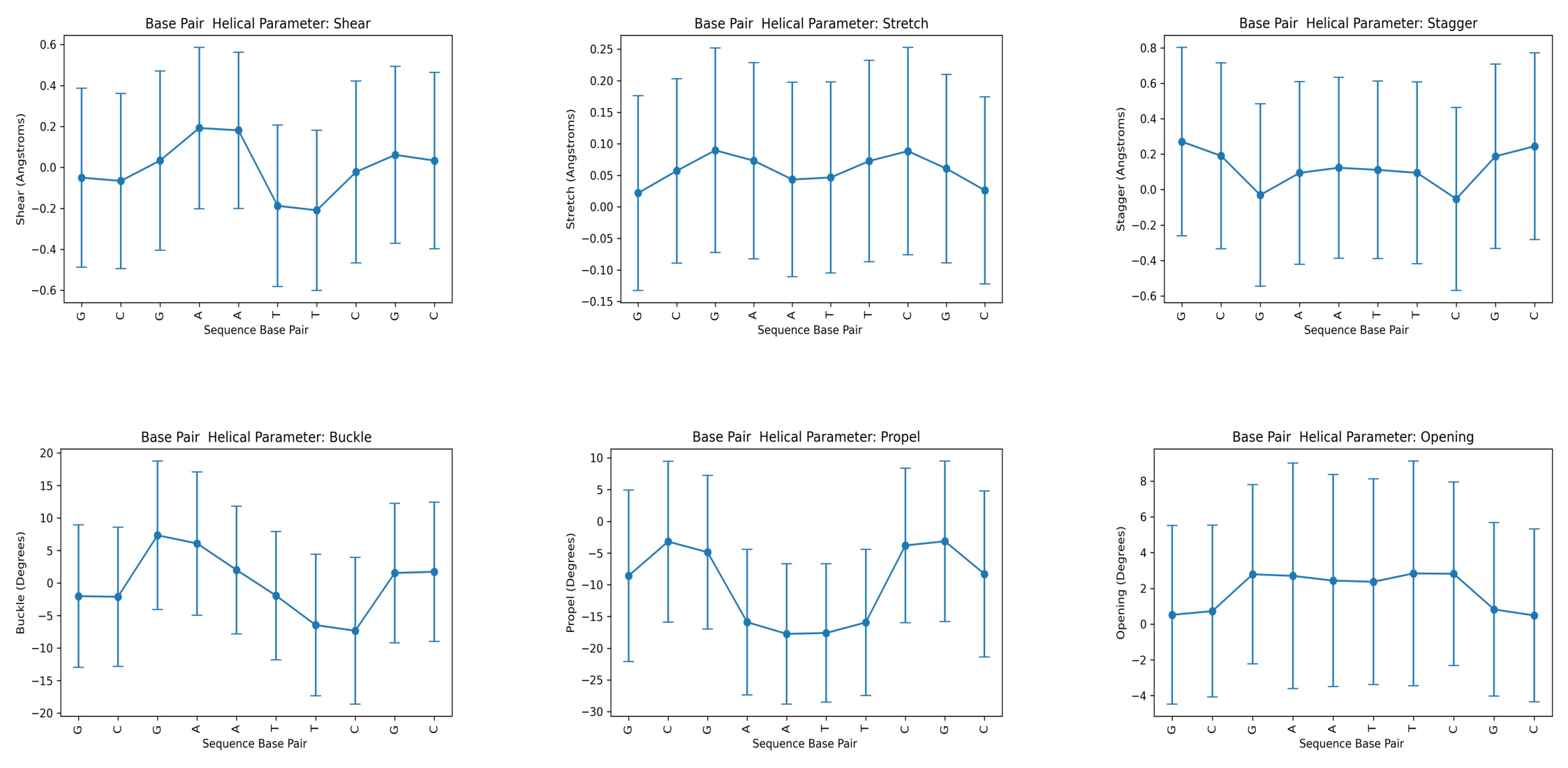
Helical Base Pair (Intra Base Pair) Parameters

Translational (Shear, Stretch, Stagger) and rotational (Buckle, Propeller, Opening) parameters related to a dinucleotide Intra-Base Pair.

• Shear: Translation around the X-axis.

• Stretch: Translation around the Y-axis.

• Stagger: Translation around the Z-axis.

• Buckle: Rotation around the X-axis.

• Propeller: Rotation around the Y-axis.

• Opening: Rotation around the Z-axis.

---

---

Building Block used:

• dna_averages from biobb_dna.dna.dna_averages

---

Computing average values from all base-pair parameters

from biobb_dna.dna.dna_averages import dna_averages

for helpar in base_pair:

    #input_file_path = canal_out + "_" + helpar + ".ser"
    input_file_path = "canal_out/canal_output" + "_" + helpar + ".ser"
    output_averages_csv_path= helpar+'.averages.csv'
    output_averages_jpg_path= helpar+'.averages.jpg'

    prop = {
        'helpar_name': helpar,
        'sequence': seq
    }

    dna_averages(
        input_ser_path=input_file_path,
        output_csv_path=output_averages_csv_path,
        output_jpg_path=output_averages_jpg_path,
        properties=prop)

Showing the calculated average values for all base-pair helical parameters

for helpar in base_pair:
    output_averages_csv_path= helpar+'.averages.csv'
    df = pd.read_csv(output_averages_csv_path)
    print("Helical Parameter: " + helpar)
    print(df)
    print("---------\n")

Helical Parameter: shear
  Base Pair       mean       std
0          G -0.049992  0.437419
1          C -0.066120  0.428450
2          G  0.033414  0.438027
3          A  0.192408  0.393915
4          A  0.181268  0.382112
5          T -0.187710  0.394140
6          T -0.209416  0.391508
7          C -0.021976  0.444251
8          G  0.061500  0.432066
9          C  0.033314  0.430674
---------

Helical Parameter: stretch
  Base Pair       mean       std
0          G  0.021910  0.154373
1          C  0.057128  0.146271
2          G  0.089684  0.162121
3          A  0.073182  0.155722
4          A  0.043370  0.154155
5          T  0.046586  0.151565
6          T  0.072776  0.159554
7          C  0.088406  0.164430
8          G  0.060682  0.149506
9          C  0.026160  0.148136
---------

Helical Parameter: stagger
  Base Pair       mean       std
0          G  0.270900  0.531987
1          C  0.190716  0.524902
2          G -0.030574  0.514709
3          A  0.094458  0.515384
4          A  0.123512  0.511518
5          T  0.111454  0.501179
6          T  0.094714  0.513247
7          C -0.052344  0.516656
8          G  0.187962  0.520935
9          C  0.245116  0.527218
---------

Helical Parameter: buckle
  Base Pair       mean        std
0          G -2.011124  10.957743
1          C -2.108248  10.706547
2          G  7.351526  11.411534
3          A  6.094836  11.016860
4          A  2.021262   9.824963
5          T -1.932570   9.869768
6          T -6.454566  10.888373
7          C -7.332888  11.269869
8          G  1.551400  10.722523
9          C  1.740906  10.696502
---------

Helical Parameter: propel
  Base Pair        mean        std
0          G  -8.589338  13.487527
1          C  -3.200962  12.673929
2          G  -4.877606  12.107475
3          A -15.895916  11.463353
4          A -17.740540  11.053182
5          T -17.600944  10.901201
6          T -15.934650  11.522282
7          C  -3.809752  12.151864
8          G  -3.145238  12.632066
9          C  -8.300600  13.082747
---------

Helical Parameter: opening
  Base Pair       mean       std
0          G  0.519980  4.990688
1          C  0.727574  4.801118
2          G  2.788520  5.011118
3          A  2.696966  6.306307
4          A  2.434002  5.929345
5          T  2.367904  5.751322
6          T  2.837478  6.282682
7          C  2.813492  5.139189
8          G  0.822494  4.850359
9          C  0.483850  4.838646
---------

Plotting the average values for all base-pair helical parameters

images = []
for helpar in base_pair:
    images.append(helpar + '.averages.jpg')

f, axarr = plt.subplots(2, 3, figsize=(40, 20))

for i, image in enumerate(images):
    y = i%3
    x = int(i/3)

    img = mpimg.imread(image)

    axarr[x,y].imshow(img, aspect='auto')
    axarr[x,y].axis('off')

plt.show()

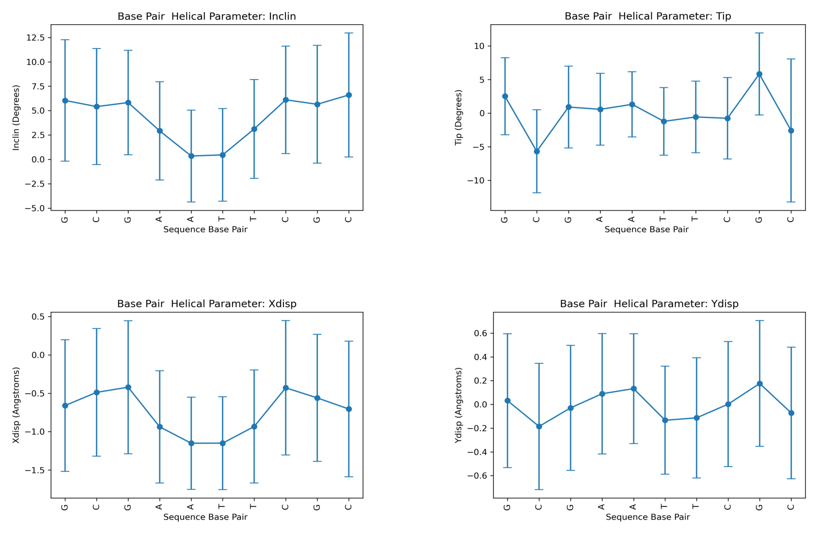
Axis Base Pair Parameters

---

Translational (x/y-displacement) and rotational (inclination, tip) parameters related to a dinucleotide Base Pair.

• X-displacement: Translation around the X-axis.

• Y-displacement: Translation around the Y-axis.

• Inclination: Rotation around the X-axis.

• Tip: Rotation around the Y-axis.

---

---

Building Block used:

• dna_averages from biobb_dna.dna.averages

---

Computing average values from all Axis base-pair parameters

from biobb_dna.dna.dna_averages import dna_averages

for helpar in axis_base_pairs:

    #input_file_path = canal_out + "_" + helpar + ".ser"
    input_file_path = "canal_out/canal_output" + "_" + helpar + ".ser"
    output_averages_csv_path= helpar+'.averages.csv'
    output_averages_jpg_path= helpar+'.averages.jpg'

    prop = {
        'helpar_name': helpar,
        'sequence': seq,
#        'seqpos': [4,3]
    }

    dna_averages(
        input_ser_path=input_file_path,
        output_csv_path=output_averages_csv_path,
        output_jpg_path=output_averages_jpg_path,
        properties=prop)

Showing the calculated average values for all Axis base-pair helical parameters

for helpar in axis_base_pairs:
    output_averages_csv_path= helpar+'.averages.csv'
    df = pd.read_csv(output_averages_csv_path)
    print("Helical Parameter: " + helpar)
    print(df)
    print("---------\n")

Helical Parameter: inclin
  Base Pair       mean       std
0          G  6.041284  6.230831
1          C  5.410818  5.944490
2          G  5.825528  5.359376
3          A  2.924440  5.031021
4          A  0.346356  4.709278
5          T  0.460490  4.744693
6          T  3.120780  5.069334
7          C  6.106598  5.504673
8          G  5.647446  6.043921
9          C  6.601924  6.358550
---------

Helical Parameter: tip
  Base Pair       mean        std
0          G  2.512608   5.728359
1          C -5.681794   6.177066
2          G  0.907828   6.084601
3          A  0.569286   5.347552
4          A  1.306582   4.845978
5          T -1.227768   5.019692
6          T -0.568284   5.338846
7          C -0.767708   6.048420
8          G  5.821194   6.102313
9          C -2.578986  10.627202
---------

Helical Parameter: xdisp
  Base Pair       mean       std
0          G -0.659664  0.857688
1          C -0.487874  0.832502
2          G -0.421234  0.867164
3          A -0.937412  0.731117
4          A -1.150654  0.600304
5          T -1.149698  0.604352
6          T -0.933022  0.736415
7          C -0.428964  0.875973
8          G -0.560260  0.827803
9          C -0.704972  0.883845
---------

Helical Parameter: ydisp
  Base Pair       mean       std
0          G  0.031522  0.563973
1          C -0.185588  0.531173
2          G -0.029302  0.526326
3          A  0.089948  0.507185
4          A  0.132712  0.462237
5          T -0.133432  0.454954
6          T -0.113044  0.506105
7          C  0.002278  0.526475
8          G  0.176116  0.529698
9          C -0.071754  0.554503
---------

Plotting the average values for all Axis base-pair helical parameters

images = []
for helpar in axis_base_pairs:
    images.append(helpar + '.averages.jpg')

f, axarr = plt.subplots(2, 2, figsize=(30, 20))

for i, image in enumerate(images):
    y = i%2
    x = int(i/2)

    img = mpimg.imread(image)

    axarr[x,y].imshow(img, aspect='auto')
    axarr[x,y].axis('off')

plt.show()

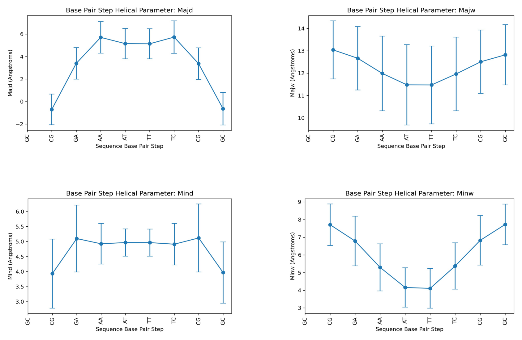
Grooves

---

Nucleic Acid Structure’s strand backbones appear closer together on one side of the helix than on the other. This creates a Major groove (where backbones are far apart) and a Minor groove (where backbones are close together). Depth and width of these grooves can be mesured giving information about the different conformations that the nucleic acid structure can achieve.

• Major Groove Width.

• Major Groove Depth.

• Minor Groove Width.

• Minor Groove Depth.

---

---

Building Block used:

• dna_averages from biobb_dna.dna.dna_averages

---

Computing average values from all Grooves parameters

from biobb_dna.dna.dna_averages import dna_averages

for helpar in grooves:

    #input_file_path = canal_out + "_" + helpar + ".ser"
    input_file_path = "canal_out/canal_output" + "_" + helpar + ".ser"
    output_averages_csv_path= helpar+'.averages.csv'
    output_averages_jpg_path= helpar+'.averages.jpg'

    prop = {
        'helpar_name': helpar,
        'sequence': seq
    }

    dna_averages(
        input_ser_path=input_file_path,
        output_csv_path=output_averages_csv_path,
        output_jpg_path=output_averages_jpg_path,
        properties=prop)

Showing the calculated average values for all Grooves parameters

for helpar in grooves:
    output_averages_csv_path= helpar+'.averages.csv'
    df = pd.read_csv(output_averages_csv_path)
    print("Helical Parameter: " + helpar)
    print(df)
    print("---------\n")

Helical Parameter: majd
  Base Pair Step      mean       std
0             GC       NaN       NaN
1             CG -0.703077  1.362241
2             GA  3.396398  1.402178
3             AA  5.710123  1.406443
4             AT  5.156143  1.346752
5             TT  5.139702  1.337523
6             TC  5.735556  1.447770
7             CG  3.371511  1.402279
8             GC -0.644086  1.444480
---------

Helical Parameter: majw
  Base Pair Step       mean       std
0             GC        NaN       NaN
1             CG  13.040615  1.300370
2             GA  12.664800  1.419105
3             AA  11.986143  1.670021
4             AT  11.476450  1.797558
5             TT  11.472435  1.740485
6             TC  11.964836  1.648435
7             CG  12.508447  1.419017
8             GC  12.819785  1.347786
---------

Helical Parameter: mind
  Base Pair Step      mean       std
0             GC       NaN       NaN
1             CG  3.932224  1.148757
2             GA  5.100660  1.114656
3             AA  4.926210  0.677415
4             AT  4.968002  0.453657
5             TT  4.966188  0.452291
6             TC  4.912856  0.690885
7             CG  5.121034  1.132328
8             GC  3.969312  1.021299
---------

Helical Parameter: minw
  Base Pair Step      mean       std
0             GC       NaN       NaN
1             CG  7.713347  1.175525
2             GA  6.789962  1.405118
3             AA  5.296306  1.332686
4             AT  4.160776  1.113765
5             TT  4.109198  1.119448
6             TC  5.376128  1.314328
7             CG  6.827374  1.402630
8             GC  7.729192  1.148585
---------

Plotting the average values for all Grooves helical parameters

images = []
for helpar in grooves:
    images.append(helpar + '.averages.jpg')

f, axarr = plt.subplots(2, 2, figsize=(30, 20))

for i, image in enumerate(images):
    y = i%2
    x = int(i/2)

    img = mpimg.imread(image)

    axarr[x,y].imshow(img, aspect='auto')
    axarr[x,y].axis('off')

plt.show()

Backbone Torsions

---

The three major elements of flexibility in the backbone are:

• Sugar Puckering:

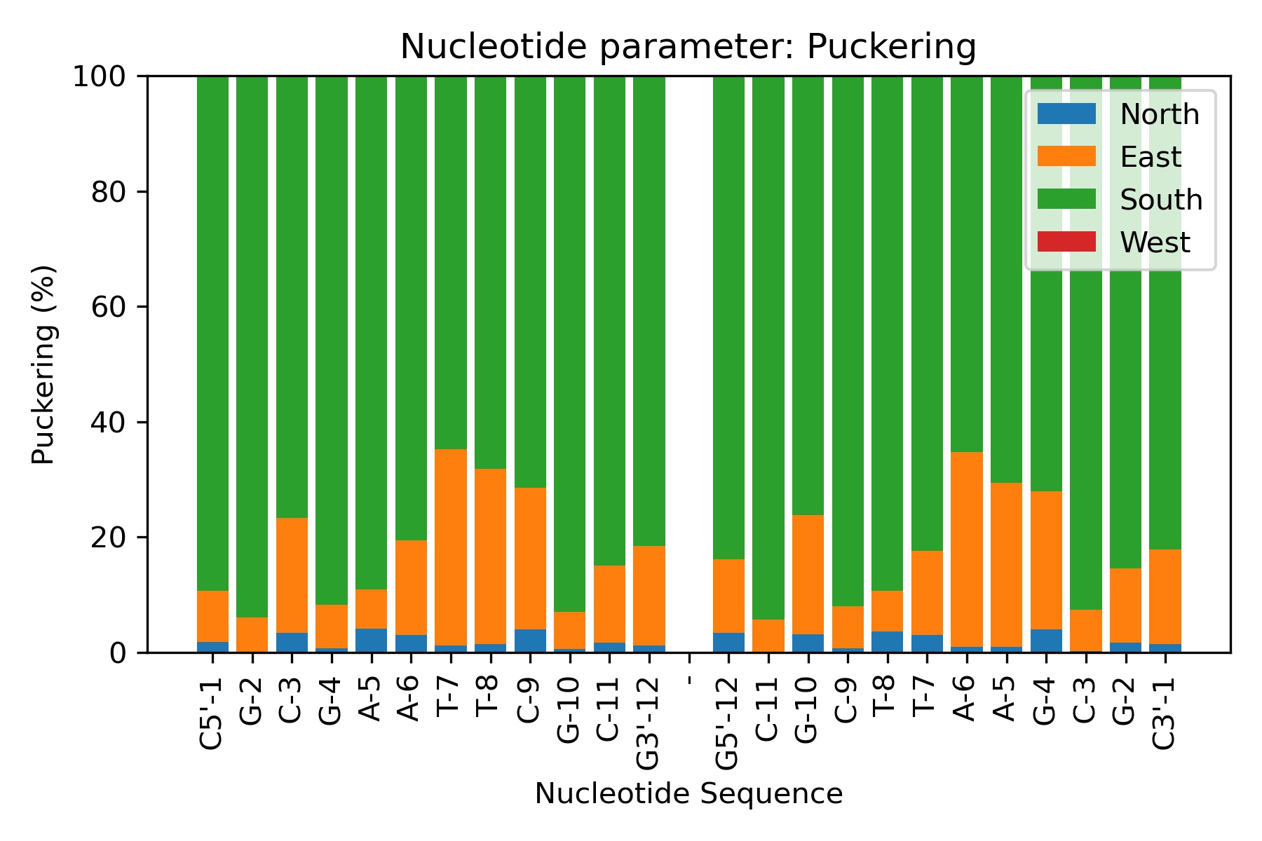
  Sugar Puckering annotation is done by dividing the pseudo-rotational circle in four equivalent sections:
  
  

  • North: 315:45º

  • East: 45:135º

  • South: 135:225º

  • West: 225:315º

These four conformations are those dominating sugar conformational space, in agreement with all available experimental data.

• Canonical Alpha/Gamma:

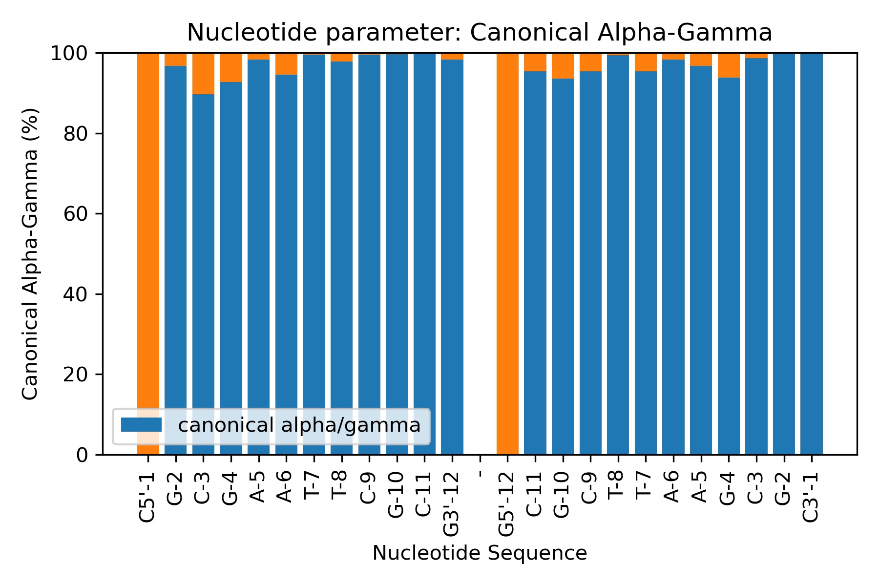
  Rotations around α/γ torsions generate non-canonical local conformations leading to a reduced twist and they have been reported as being important in the formation of several protein-DNA complexes.

• BI/BII Population:

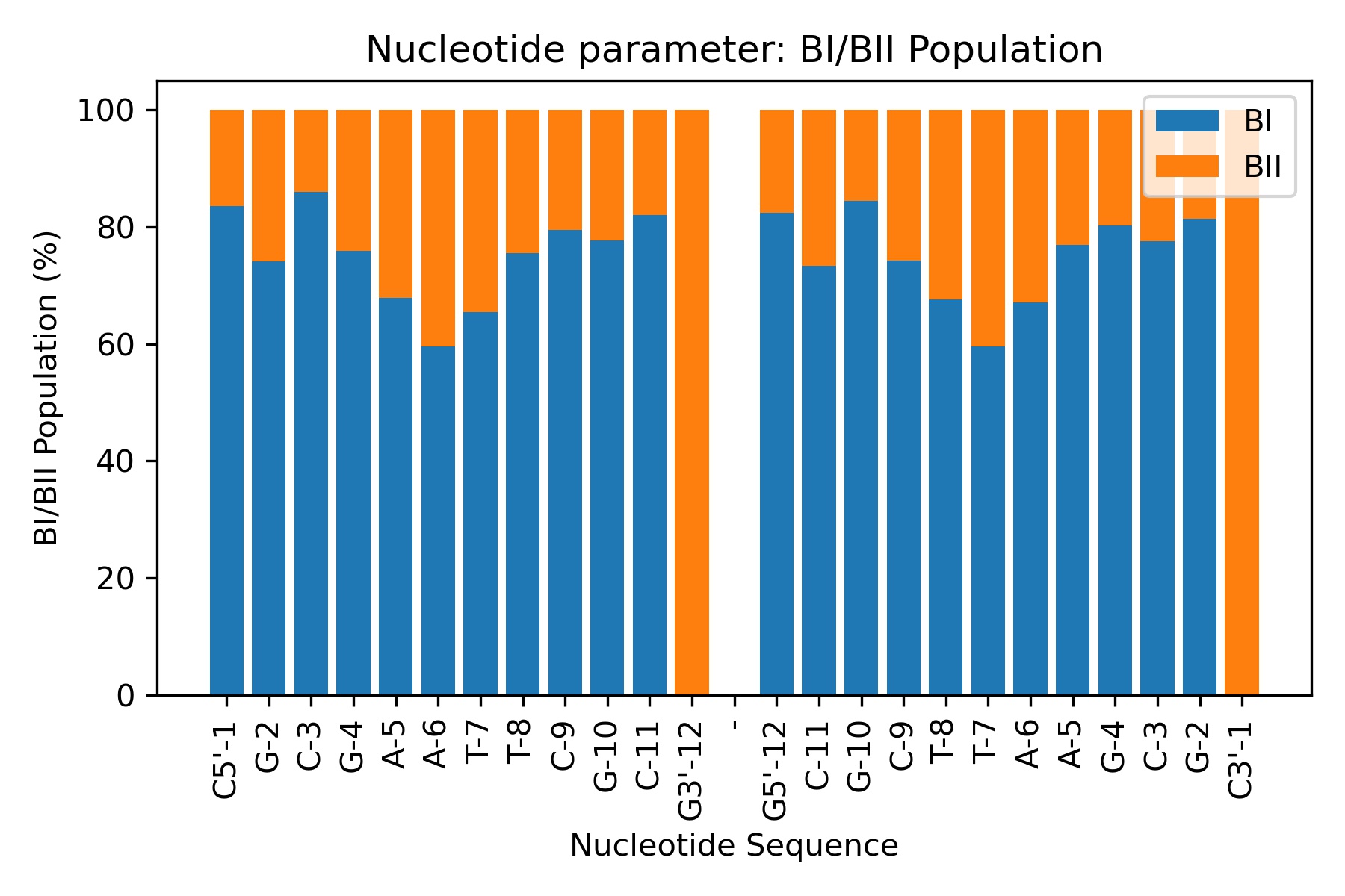
  The concerted rotation around ζ/ε torsions generates two major conformers: BI and BII, which are experimentally known to co-exist in a ratio around 80%:20% (BI:BII) in B-DNA.

Sugar Puckering	Canonical Alpha/Gamma	BI/BII population

---

Building Blocks used:

• puckering from biobb_dna.backbone.puckering

• canonicalag from biobb_dna.backbone.canonicalag

• bipopulations from biobb_dna.backbone.bipopulations

---

Sugar Puckering

Computing average values

from biobb_dna.backbone.puckering import puckering

canal_phaseC = "canal_out/canal_output_phaseC.ser"
canal_phaseW = "canal_out/canal_output_phaseW.ser"

output_puckering_csv_path = 'puckering.averages.csv'
output_puckering_jpg_path = 'puckering.averages.jpg'

prop = {
    'sequence': seq
}

puckering(
    input_phaseC_path=canal_phaseC,
    input_phaseW_path=canal_phaseW,
    output_csv_path=output_puckering_csv_path,
    output_jpg_path=output_puckering_jpg_path,
    properties=prop)

Showing the calculated average values

df = pd.read_csv(output_puckering_csv_path)
df

	Nucleotide	North	East	West	South
0	C5'-1	1.82	8.84	0.02	89.32
1	G-2	0.10	5.92	0.02	93.96
2	C-3	3.36	20.02	0.00	76.60
3	G-4	0.76	7.52	0.00	91.72
4	A-5	4.16	6.72	0.00	89.10
5	A-6	3.04	16.44	0.00	80.50
6	T-7	1.16	34.06	0.00	64.76
7	T-8	1.50	30.36	0.00	68.10
8	C-9	4.00	24.56	0.00	71.44
9	G-10	0.60	6.40	0.02	92.98
10	C-11	1.72	13.38	0.00	84.90
11	G3'-12	1.18	17.28	0.04	81.50
12	-	0.00	0.00	0.00	0.00
13	G5'-12	3.44	12.72	0.02	83.80
14	C-11	0.16	5.56	0.00	94.24
15	G-10	3.14	20.70	0.00	76.14
16	C-9	0.70	7.32	0.00	91.98
17	T-8	3.64	7.04	0.00	89.32
18	T-7	3.02	14.58	0.02	82.38
19	A-6	0.96	33.82	0.00	65.22
20	A-5	1.00	28.42	0.00	70.58
21	G-4	4.00	23.96	0.02	71.98
22	C-3	0.24	7.14	0.02	92.60
23	G-2	1.72	12.86	0.00	85.40
24	C3'-1	1.40	16.46	0.00	82.12

Plotting the average values

Image(filename=output_puckering_jpg_path,width = 600)

Canonical Alpha/Gamma

Computing average values

from biobb_dna.backbone.canonicalag import canonicalag

canal_alphaC = "canal_out/canal_output_alphaC.ser"
canal_alphaW = "canal_out/canal_output_alphaW.ser"
canal_gammaC = "canal_out/canal_output_gammaC.ser"
canal_gammaW = "canal_out/canal_output_gammaW.ser"

output_alphagamma_csv_path = 'alphagamma.averages.csv'
output_alphagamma_jpg_path = 'alphagamma.averages.jpg'

prop = {
    'sequence': seq
}

canonicalag(
    input_alphaC_path=canal_alphaC,
    input_alphaW_path=canal_alphaW,
    input_gammaC_path=canal_gammaC,
    input_gammaW_path=canal_gammaW,
    output_csv_path=output_alphagamma_csv_path,
    output_jpg_path=output_alphagamma_jpg_path,
    properties=prop)

Showing the calculated average values

df = pd.read_csv(output_alphagamma_csv_path)
df

	Nucleotide	Canonical alpha/gamma
0	C5'-1	0.00
1	G-2	96.76
2	C-3	89.66
3	G-4	92.70
4	A-5	98.30
5	A-6	94.52
6	T-7	99.56
7	T-8	97.86
8	C-9	99.54
9	G-10	99.64
10	C-11	99.72
11	G3'-12	98.24
12	-	0.00
13	G5'-12	0.00
14	C-11	95.42
15	G-10	93.56
16	C-9	95.40
17	T-8	99.38
18	T-7	95.36
19	A-6	98.28
20	A-5	96.70
21	G-4	93.86
22	C-3	98.70
23	G-2	100.00
24	C3'-1	99.78

Plotting the average values

Image(filename=output_alphagamma_jpg_path,width = 600)

BI/BII Population

Computing average values

from biobb_dna.backbone.bipopulations import bipopulations

canal_epsilC = "canal_out/canal_output_epsilC.ser"
canal_epsilW = "canal_out/canal_output_epsilW.ser"
canal_zetaC = "canal_out/canal_output_zetaC.ser"
canal_zetaW = "canal_out/canal_output_zetaW.ser"

output_bIbII_csv_path = 'bIbII.averages.csv'
output_bIbII_jpg_path = 'bIbII.averages.jpg'

prop = {
    'sequence': seq
}

bipopulations(
    input_epsilC_path=canal_epsilC,
    input_epsilW_path=canal_epsilW,
    input_zetaC_path=canal_zetaC,
    input_zetaW_path=canal_zetaW,
    output_csv_path=output_bIbII_csv_path,
    output_jpg_path=output_bIbII_jpg_path,
    properties=prop)

Showing the calculated average values

df = pd.read_csv(output_bIbII_csv_path)
df

	Nucleotide	BI population	BII population
0	C5'-1	83.523295	16.476705
1	G-2	74.085183	25.914817
2	C-3	85.982803	14.017197
3	G-4	75.924815	24.075185
4	A-5	67.846431	32.153569
5	A-6	59.588082	40.411918
6	T-7	65.406919	34.593081
7	T-8	75.524895	24.475105
8	C-9	79.504099	20.495901
9	G-10	77.644471	22.355529
10	C-11	82.003599	17.996401
11	G3'-12	0.000000	100.000000
12	-	0.000000	100.000000
13	G5'-12	82.443511	17.556489
14	C-11	73.305339	26.694661
15	G-10	84.483103	15.516897
16	C-9	74.305139	25.694861
17	T-8	67.606479	32.393521
18	T-7	59.568086	40.431914
19	A-6	67.126575	32.873425
20	A-5	76.984603	23.015397
21	G-4	80.243951	19.756049
22	C-3	77.604479	22.395521
23	G-2	81.443711	18.556289
24	C3'-1	0.000000	100.000000

Plotting the average values

Image(filename=output_bIbII_jpg_path,width = 600)

Extracting Time series Helical Parameters

Time series values for the set of helical parameters can be also extracted from the output of Curves+/Canal execution on Molecular Dynamics Trajectories. The helical parameters can be divided in the same 5 main blocks previously introduced:

• Helical Base Pair Step (Inter-Base Pair) Helical Parameters

• Helical Base Pair (Intra-Base Pair) Helical Parameters

• Axis Base Pair

• Grooves

• Backbone Torsions

---

Building Block used:

• dna_timeseries from biobb_dna.dna.dna_timeseries

---

Extracting a particular Helical Parameter

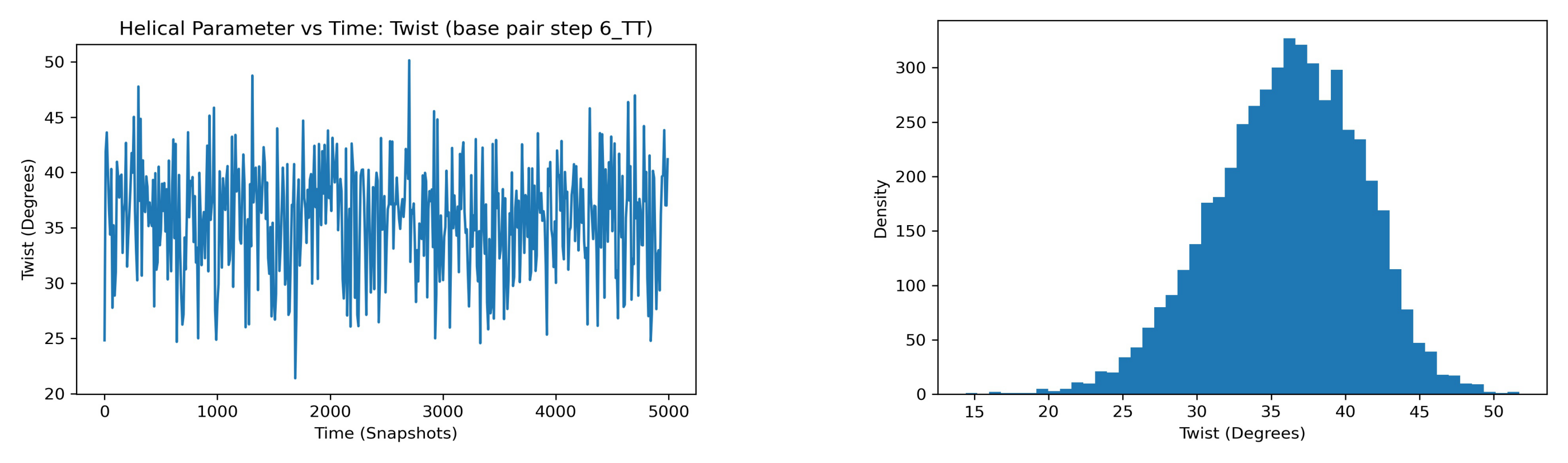
Time series values can be extracted from any of the helical parameters previously introduced. To illustrate the steps needed, the base-pair step helical parameter Twist has been selected. Please note that computing the time series values for a different helical parameter just requires modifying the helpar variable from the next cell.

from biobb_dna.dna.dna_timeseries import dna_timeseries

# Modify the next variable to extract time series values for a different helical parameter
# Possible values are: 
    # Base Pair Step (Inter Base Pair) Helical Parameters: shift, slide, rise, tilt, roll, twist 
    # Base Pair (Intra Base Pair) Helical Parameters: shear, stretch, stagger, buckle, propeller, opening
    # Axis Parameters: inclin, tip, xdisp, ydisp
    # Backbone Torsions Parameters: alphaC, alphaW, betaC, betaW, gammaC, gammaW, deltaC, deltaW,
    #                                epsilC, epsilW, zetaC, zetaW, chiC, chiW, phaseC, phaseW
    # Grooves: mind, minw, majd, majw

helpar = "twist" # Modify this variable to extract time series values for a different helical parameter

input_file_path = "canal_out/canal_output" + "_" + helpar + ".ser"
output_timeseries_file_path = helpar + '.timeseries.zip'

prop = {
    'helpar_name': helpar,
    'sequence': seq
}

dna_timeseries(
    input_ser_path=input_file_path,
    output_zip_path=output_timeseries_file_path,
    properties=prop)

Extracting time series results for the selected helical parameter in a temporary folder

timeseries_dir = "timeseries"

if Path(timeseries_dir).exists(): shutil.rmtree(timeseries_dir) 
os.mkdir(timeseries_dir)

with zipfile.ZipFile(output_timeseries_file_path, 'r') as zip_ref:
    zip_ref.extractall(timeseries_dir)

Finding out all the possible nucleotide / base / base-pair / base-pair steps

Discover all the possible nucleotide / base / base-pair / base-pair steps from the sequence. The unit will depend on the helical parameter being studied.
Select one of them to study the time series values of the helical parameter along the simulation.

helpartimesfiles = glob.glob(timeseries_dir + "/*series*.csv") 

helpartimes = []
for file in helpartimesfiles:
    new_string = file.replace(timeseries_dir + "/series_" + helpar + "_", "")
    new_string = new_string.replace(".csv" , "")
    helpartimes.append(new_string)
    
timesel = ipywidgets.Dropdown(
    options=helpartimes,
    description='Sel. BPS:',
    disabled=False,
)
display(timesel)

Showing the time series values for the selected unit

file_ser = timeseries_dir + "/series_" + helpar + "_" + timesel.value + ".csv"

df = pd.read_csv(file_ser)
df

	Unnamed: 0	6_TT
0	0	24.83
1	1	36.78
2	2	41.00
3	3	33.50
4	4	29.68
...	...	...
4995	4995	42.40
4996	4996	44.61
4997	4997	39.61
4998	4998	36.93
4999	4999	36.63

5000 rows × 2 columns

file_hist = timeseries_dir + "/hist_" + helpar + "_" + timesel.value + ".csv"

df = pd.read_csv(file_hist)
df

	twist	density
0	14.410000	1.0
1	15.203617	0.0
2	15.997234	2.0
3	16.790851	1.0
4	17.584468	1.0
5	18.378085	1.0
6	19.171702	5.0
7	19.965319	3.0
8	20.758936	5.0
9	21.552553	11.0
10	22.346170	10.0
11	23.139787	21.0
12	23.933404	20.0
13	24.727021	34.0
14	25.520638	43.0
15	26.314255	61.0
16	27.107872	80.0
17	27.901489	91.0
18	28.695106	114.0
19	29.488723	138.0
20	30.282340	176.0
21	31.075957	181.0
22	31.869574	208.0
23	32.663191	248.0
24	33.456809	265.0
25	34.250426	280.0
26	35.044043	300.0
27	35.837660	327.0
28	36.631277	321.0
29	37.424894	304.0
30	38.218511	270.0
31	39.012128	298.0
32	39.805745	243.0
33	40.599362	234.0
34	41.392979	196.0
35	42.186596	169.0
36	42.980213	115.0
37	43.773830	78.0
38	44.567447	47.0
39	45.361064	39.0
40	46.154681	18.0
41	46.948298	17.0
42	47.741915	10.0
43	48.535532	9.0
44	49.329149	2.0
45	50.122766	1.0
46	50.916383	2.0

Plotting the time series values for the selected base-pair step

file_ser = timeseries_dir + "/series_" + helpar + "_" + timesel.value + ".jpg"
file_hist = timeseries_dir + "/hist_" + helpar + "_" + timesel.value + ".jpg"

images = []

images.append(file_ser)
images.append(file_hist)

f, axarr = plt.subplots(1, 2, figsize=(50, 15))

for i, image in enumerate(images):
    img = mpimg.imread(image)

    axarr[i].imshow(img, aspect='auto')
    axarr[i].axis('off')

plt.show()

Computing timeseries for all base-pair step parameters

from biobb_dna.dna.dna_timeseries import dna_timeseries

output_timeseries_bps_file_paths = {}
for helpar in base_pair_step:

    input_file_path = "canal_out/canal_output" + "_" + helpar + ".ser"
    output_timeseries_bps_file_paths[helpar] = helpar + '.timeseries.zip'

    prop = {
        'helpar_name': helpar,
        'sequence': seq
    }

    dna_timeseries(
        input_ser_path=input_file_path,
        output_zip_path=output_timeseries_bps_file_paths[helpar],
        properties=prop)

#if Path(timeseries_dir).exists(): shutil.rmtree(timeseries_dir) 
#os.mkdir(timeseries_dir)

for timeseries_zipfile in output_timeseries_bps_file_paths.values():
    with zipfile.ZipFile(timeseries_zipfile, 'r') as zip_ref:
        zip_ref.extractall(timeseries_dir)

Computing timeseries for all base-pair parameters

from biobb_dna.dna.dna_timeseries import dna_timeseries

output_timeseries_bp_file_paths = {}
for helpar in base_pair:

    input_file_path = "canal_out/canal_output" + "_" + helpar + ".ser"
    output_timeseries_bp_file_paths[helpar] = helpar + '.timeseries.zip'

    prop = {
        'helpar_name': helpar,
        'sequence': seq
    }

    dna_timeseries(
        input_ser_path=input_file_path,
        output_zip_path=output_timeseries_bp_file_paths[helpar],
        properties=prop)

#if Path(timeseries_dir).exists(): shutil.rmtree(timeseries_dir) 
#os.mkdir(timeseries_dir)

for timeseries_zipfile in output_timeseries_bp_file_paths.values():
    with zipfile.ZipFile(timeseries_zipfile, 'r') as zip_ref:
        zip_ref.extractall(timeseries_dir)

Computing timeseries for all axis parameters

from biobb_dna.dna.dna_timeseries import dna_timeseries

output_timeseries_bp_file_paths = {}
for helpar in axis_base_pairs:

    input_file_path = "canal_out/canal_output" + "_" + helpar + ".ser"
    output_timeseries_bp_file_paths[helpar] = helpar + '.timeseries.zip'

    prop = {
        'helpar_name': helpar,
        'sequence': seq
    }

    dna_timeseries(
        input_ser_path=input_file_path,
        output_zip_path=output_timeseries_bp_file_paths[helpar],
        properties=prop)

for timeseries_zipfile in output_timeseries_bp_file_paths.values():
    with zipfile.ZipFile(timeseries_zipfile, 'r') as zip_ref:
        zip_ref.extractall(timeseries_dir)

Computing timeseries for all grooves parameters

from biobb_dna.dna.dna_timeseries import dna_timeseries

output_timeseries_bp_file_paths = {}
for helpar in grooves:

    input_file_path = "canal_out/canal_output" + "_" + helpar + ".ser"
    output_timeseries_bp_file_paths[helpar] = helpar + '.timeseries.zip'

    prop = {
        'helpar_name': helpar,
        'sequence': seq
    }

    dna_timeseries(
        input_ser_path=input_file_path,
        output_zip_path=output_timeseries_bp_file_paths[helpar],
        properties=prop)

for timeseries_zipfile in output_timeseries_bp_file_paths.values():
    with zipfile.ZipFile(timeseries_zipfile, 'r') as zip_ref:
        zip_ref.extractall(timeseries_dir)

Computing timeseries for all backbone torsions parameters

from biobb_dna.dna.dna_timeseries import dna_timeseries

output_timeseries_bp_file_paths = {}
for helpar in backbone_torsions:

    input_file_path = "canal_out/canal_output" + "_" + helpar + ".ser"
    output_timeseries_bp_file_paths[helpar] = helpar + '.timeseries.zip'

    prop = {
        'helpar_name': helpar,
        'sequence': seq
    }

    dna_timeseries(
        input_ser_path=input_file_path,
        output_zip_path=output_timeseries_bp_file_paths[helpar],
        properties=prop)

for timeseries_zipfile in output_timeseries_bp_file_paths.values():
    with zipfile.ZipFile(timeseries_zipfile, 'r') as zip_ref:
        zip_ref.extractall(timeseries_dir)

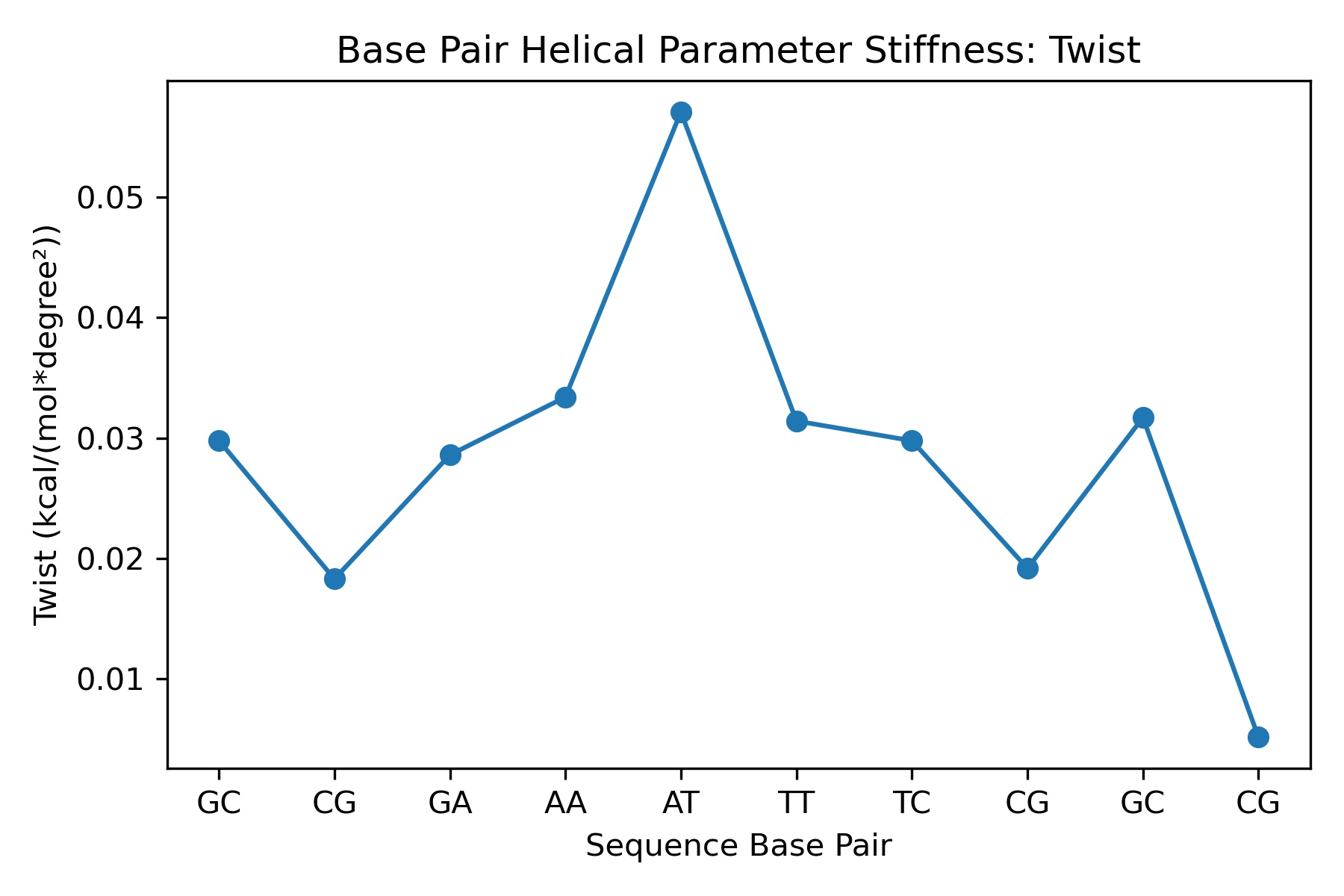
Stiffness

Molecular stiffness is an elastic force constant associated with helical deformation at the base pair step level and is determined by inversion of the covariance matrix in helical space, which yields stiffness matrices whose diagonal elements provide the stiffness constants associated with pure rotational (twist, roll and tilt) and translational (rise, shift and slide) deformations within the given step.

---

---

Building Blocks used:

• average_stiffness from biobb_dna.stiffness.average_stiffness

• basepair_stiffness from biobb_dna.stiffness.basepair_stiffness

---

from biobb_dna.stiffness.average_stiffness import average_stiffness

helpar = "twist" # Modify this variable to extract time series values for a different helical parameter

input_file_path = "canal_out/canal_output" + "_" + helpar + ".ser"
output_stiffness_csv_path = helpar + '.stiffness.csv'
output_stiffness_jpg_path = helpar + '.stiffness.jpg'

prop = { 
    'sequence' : seq
}

average_stiffness(
    input_ser_path=input_file_path,
    output_csv_path=output_stiffness_csv_path,
    output_jpg_path=output_stiffness_jpg_path,
    properties=prop)

df = pd.read_csv(output_stiffness_csv_path)
df

	Unnamed: 0	twist_stiffness
0	GC	0.029784
1	CG	0.018300
2	GA	0.028595
3	AA	0.033391
4	AT	0.057062
5	TT	0.031410
6	TC	0.029772
7	CG	0.019181
8	GC	0.031688
9	CG	0.005167

Image(filename=output_stiffness_jpg_path,width = 600)

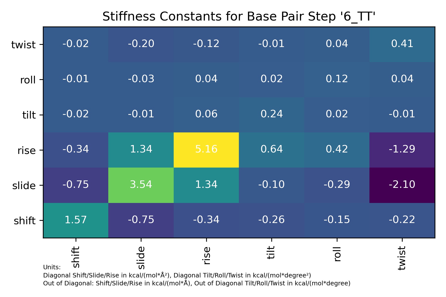
from biobb_dna.stiffness.basepair_stiffness import basepair_stiffness

timeseries_shift = timeseries_dir+"/series_shift_" + timesel.value + ".csv"
timeseries_slide = timeseries_dir+"/series_slide_" + timesel.value + ".csv"
timeseries_rise = timeseries_dir+"/series_rise_" + timesel.value + ".csv"
timeseries_tilt = timeseries_dir+"/series_tilt_" + timesel.value + ".csv"
timeseries_roll = timeseries_dir+"/series_roll_" + timesel.value + ".csv"
timeseries_twist = timeseries_dir+"/series_twist_" + timesel.value + ".csv"

output_stiffness_bps_csv_path = "stiffness_bps.csv"
output_stiffness_bps_jpg_path = "stiffness_bps.jpg"

basepair_stiffness(
    input_filename_shift=timeseries_shift,
    input_filename_slide=timeseries_slide,
    input_filename_rise=timeseries_rise,
    input_filename_tilt=timeseries_tilt,
    input_filename_roll=timeseries_roll,
    input_filename_twist=timeseries_twist,
    output_csv_path=output_stiffness_bps_csv_path,
    output_jpg_path=output_stiffness_bps_jpg_path)

df = pd.read_csv(output_stiffness_bps_csv_path)
df

	6_TT	shift	slide	rise	tilt	roll	twist
0	shift	1.565629	-0.750135	-0.335147	-0.263984	-0.153248	-0.220935
1	slide	-0.750135	3.535266	1.335823	-0.095199	-0.287142	-2.104566
2	rise	-0.335147	1.335823	5.158742	0.637038	0.415877	-1.293672
3	tilt	-0.024904	-0.008981	0.060098	0.235447	0.015406	-0.008404
4	roll	-0.014457	-0.027089	0.039234	0.015406	0.119149	0.038313
5	twist	-0.020843	-0.198544	-0.122045	-0.008404	0.038313	0.412179

Image(filename=output_stiffness_bps_jpg_path,width = 600)

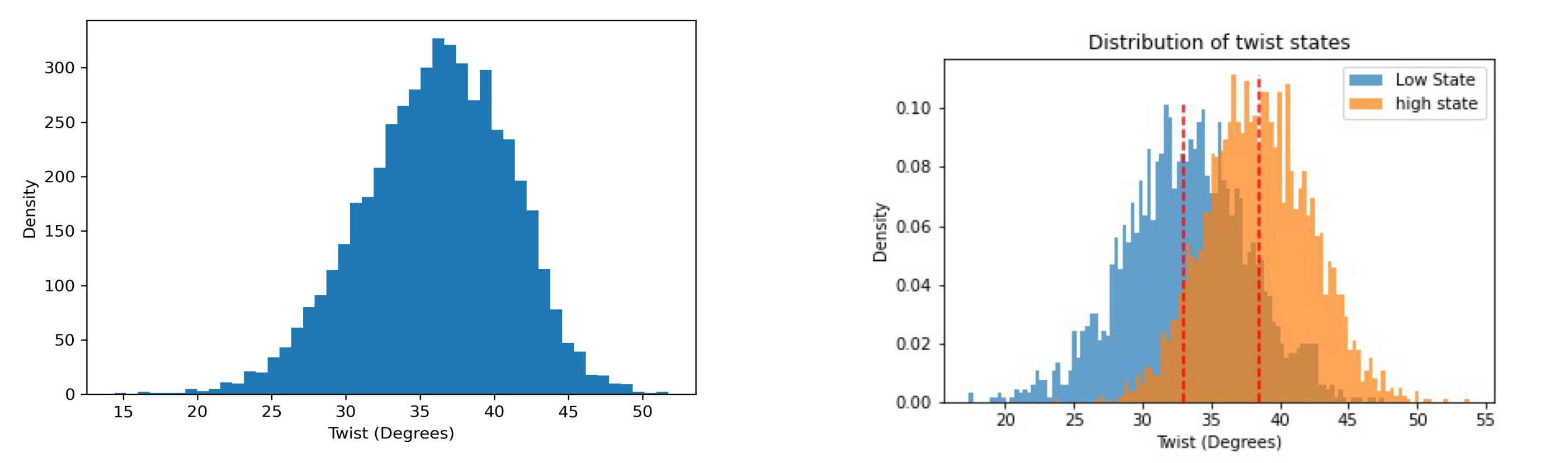
Bimodality

Base-pair steps helical parameters usually follow a normal (Gaussian-like) distribution. However, recent studies observed bimodal distributions in some base-pair steps for twist and slide, highlighting potential caveats on the harmonic approximation implicit in elastic analysis and mesoscopic models of DNA flexibility.

---

---

μABC: a systematic microsecond molecular dynamics study of tetranucleotide sequence effects in B-DNA
Marco Pasi, John H Maddocks, David Beveridge, Thomas C Bishop, David A Case, Thomas Cheatham 3rd, Pablo D Dans, B Jayaram, Filip Lankas, Charles Laughton, Jonathan Mitchell, Roman Osman, Modesto Orozco, Alberto Pérez, Daiva Petkevičiūtė, Nada Spackova, Jiri Sponer, Krystyna Zakrzewska, Richard Lavery
Nucleic Acids Research 2014, Volume 42, Issue 19, Pages 12272-12283
https://doi.org/10.1093/nar/gku855

Exploring polymorphisms in B-DNA helical conformations
Pablo D Dans, Alberto Pérez, Ignacio Faustino, Richard Lavery, Modesto Orozco
Nucleic Acids Research 2012, Volume 40, Issue 21, Pages 10668-10678
https://doi.org/10.1093/nar/gks884

A systematic molecular dynamics study of nearest-neighbor effects on base pair and base pair step conformations and fluctuations in B-DNA
Lavery R, Zakrzewska K, Beveridge D, Bishop TC, Case DA, Cheatham T, III, Dixit S, Jayaram B, Lankas F, Laughton C, John H Maddocks, Alexis Michon, Roman Osman, Modesto Orozco, Alberto Perez, Tanya Singh, Nada Spackova, Jiri Sponer
Nucleic Acids Research 2010, Volume 38, Pages 299–313
https://doi.org/10.1093/nar/gkp834

---

Building Block used:

• dna_bimodality from biobb_dna.dna.bimodality

---

from biobb_dna.dna.dna_bimodality import dna_bimodality

helpar = "twist"
input_csv = timeseries_dir+"/series_"+helpar+"_"+timesel.value+'.csv'
#input_csv = "/Users/hospital/biobb_tutorials/biobb_dna/timeseries"+"/series_"+timesel.value+'.csv' # <-- TO BE REPLACED BY PREVIOUS LINE 

output_bimodality_csv = helpar+'.bimodality.csv'
output_bimodality_jpg = helpar+'.bimodality.jpg'

prop = {
    'max_iter': 500
}
dna_bimodality(
    input_csv_file=input_csv,
    output_csv_path=output_bimodality_csv,
    output_jpg_path=output_bimodality_jpg,
    properties=prop)

file_hist = timeseries_dir + "/hist_" + helpar + "_" + timesel.value + ".jpg"
file_bi = helpar + ".bimodality.jpg"

images = []

images.append(file_hist)
images.append(file_bi)

f, axarr = plt.subplots(1, 2, figsize=(50, 15))

for i, image in enumerate(images):
    img = mpimg.imread(image)

    axarr[i].imshow(img, aspect='auto')
    axarr[i].axis('off')

plt.show()

Correlations

Sequence-dependent correlation movements have been identified in DNA conformational analysis at the base pair and base pair-step level. Trinucleotides were found to show moderate to high correlations in some intra base pair helical parameter (e.g. shear-opening, shear-stretch, stagger-buckle). Similarly, some tetranucleotides are showing strong correlations in their inter base pair helical parameters (e.g. shift-tilt, slide-twist, rise-tilt, shift-slide, and shift-twist in RR steps), with negative correlations in the shift-slide and roll-twist cases. Correlations are also observed in the combination of inter- and intra-helical parameters (e.g. shift-opening, rise-buckle, stagger-tilt). Correlations analysis can be also extended to neighboring steps (e.g. twist in the central YR step of XYRR tetranucleotides with slide in the adjacent RR step).

• Sequence Correlations: Intra-base pairs

• Sequence Correlations: Inter-base pair steps

• Helical Parameter Correlations: Intra-base pairs

• Helical Parameter Correlations: Inter-base pair steps

• Neighboring steps Correlations: Intra-base pairs

• Neighboring steps Correlations: Inter-base pair steps

---

---

The static and dynamic structural heterogeneities of B-DNA: extending Calladine–Dickerson rules
Pablo D Dans, Alexandra Balaceanu, Marco Pasi, Alessandro S Patelli, Daiva Petkevičiūtė, Jürgen Walther, Adam Hospital, Genís Bayarri, Richard Lavery, John H Maddocks, Modesto Orozco Nucleic Acids Research 2019, Volume 47, Issue 21, Pages 11090-11102
https://doi.org/10.1093/nar/gkz905

---

Building Blocks used:

• intraseqcorr from biobb_dna.intrabp_correlations.intraseqcorr

• interseqcorr from biobb_dna.interbp_correlations.interseqcorr

• intrahpcorr from biobb_dna.intrabp_correlations.intrahpcorr

• interhpcorr from biobb_dna.interbp_correlations.interhpcorr

• intrabpcorr from biobb_dna.intrabp_correlations.intrabpcorr

• interbpcorr from biobb_dna.interbp_correlations.interbpcorr

---

Sequence Correlations: Intra-base pairs

from biobb_dna.intrabp_correlations.intraseqcorr import intraseqcorr

input_file_path = "canal_out/canal_output" + "_" + helpar + ".ser"
output_intrabp_correlation_csv_path = helpar+'.intrabp_correlation.csv'
output_intrabp_correlation_jpg_path = helpar+'.intrabp_correlation.jpg'

prop={
    'sequence' : seq,
#    'helpar_name' : 'Rise'
}

intraseqcorr(
    input_ser_path=input_file_path,
    output_csv_path=output_intrabp_correlation_csv_path,
    output_jpg_path=output_intrabp_correlation_jpg_path,
    properties=prop)

df = pd.read_csv(output_intrabp_correlation_csv_path)
df

	Unnamed: 0	G	C	G_dup	A	A_dup	T	T_dup	C_dup	G_dup_dup	C_dup_dup
0	G	1.000000	-0.358404	0.068163	0.009405	0.001087	0.019698	-0.015957	0.007849	0.031577	0.010621
1	C	-0.358404	1.000000	-0.448247	-0.007771	0.026130	-0.000455	-0.005333	-0.013427	0.001874	0.025165
2	G_dup	0.068163	-0.448247	1.000000	-0.335686	-0.048327	-0.029954	0.018416	0.013668	-0.026111	0.016239
3	A	0.009405	-0.007771	-0.335686	1.000000	-0.293111	0.070316	-0.003760	0.006406	-0.000036	0.007260
4	A_dup	0.001087	0.026130	-0.048327	-0.293111	1.000000	-0.273114	-0.056474	0.001153	-0.002821	-0.016981
5	T	0.019698	-0.000455	-0.029954	0.070316	-0.273114	1.000000	-0.335193	-0.006889	-0.001462	0.017912
6	T_dup	-0.015957	-0.005333	0.018416	-0.003760	-0.056474	-0.335193	1.000000	-0.447663	0.059009	0.019932
7	C_dup	0.007849	-0.013427	0.013668	0.006406	0.001153	-0.006889	-0.447663	1.000000	-0.372677	0.014933
8	G_dup_dup	0.031577	0.001874	-0.026111	-0.000036	-0.002821	-0.001462	0.059009	-0.372677	1.000000	-0.236134
9	C_dup_dup	0.010621	0.025165	0.016239	0.007260	-0.016981	0.017912	0.019932	0.014933	-0.236134	1.000000

Image(filename=output_intrabp_correlation_jpg_path,width = 600)

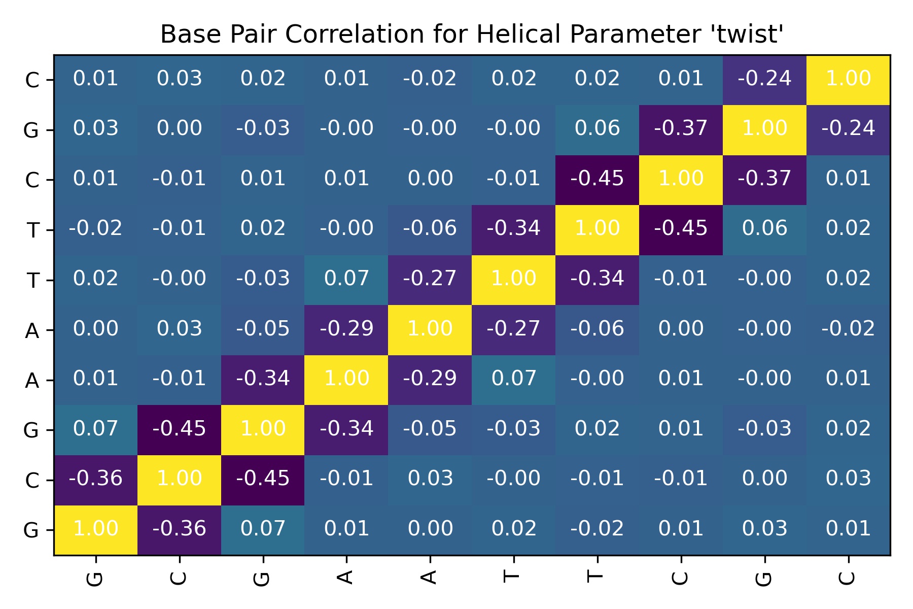
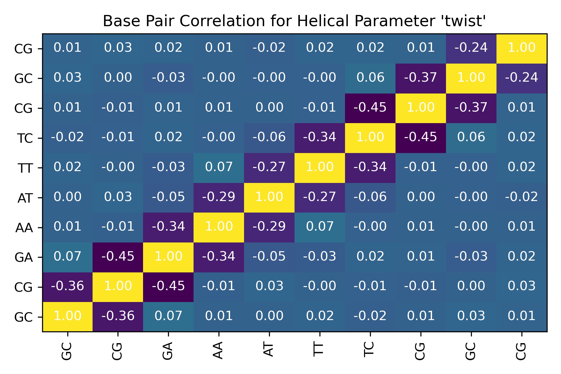
Sequence Correlations: Inter-base pair steps

from biobb_dna.interbp_correlations.interseqcorr import interseqcorr

input_file_path = "canal_out/canal_output" + "_" + helpar + ".ser"
output_interbp_correlation_csv_path = helpar+'.interbp_correlation.csv'
output_interbp_correlation_jpg_path = helpar+'.interbp_correlation.jpg'

prop={
    'sequence' : seq,
#    'helpar_name' : 'Rise'
}

interseqcorr(
    input_ser_path=input_file_path,
    output_csv_path=output_interbp_correlation_csv_path,
    output_jpg_path=output_interbp_correlation_jpg_path,
    properties=prop)

df = pd.read_csv(output_interbp_correlation_csv_path)
df

	Unnamed: 0	GC	CG	GA	AA	AT	TT	TC	CG_dup	GC_dup	CG_dup_dup
0	GC	1.000000	-0.358404	0.068163	0.009405	0.001087	0.019698	-0.015957	0.007849	0.031577	0.010621
1	CG	-0.358404	1.000000	-0.448247	-0.007771	0.026130	-0.000455	-0.005333	-0.013427	0.001874	0.025165
2	GA	0.068163	-0.448247	1.000000	-0.335686	-0.048327	-0.029954	0.018416	0.013668	-0.026111	0.016239
3	AA	0.009405	-0.007771	-0.335686	1.000000	-0.293111	0.070316	-0.003760	0.006406	-0.000036	0.007260
4	AT	0.001087	0.026130	-0.048327	-0.293111	1.000000	-0.273114	-0.056474	0.001153	-0.002821	-0.016981
5	TT	0.019698	-0.000455	-0.029954	0.070316	-0.273114	1.000000	-0.335193	-0.006889	-0.001462	0.017912
6	TC	-0.015957	-0.005333	0.018416	-0.003760	-0.056474	-0.335193	1.000000	-0.447663	0.059009	0.019932
7	CG_dup	0.007849	-0.013427	0.013668	0.006406	0.001153	-0.006889	-0.447663	1.000000	-0.372677	0.014933
8	GC_dup	0.031577	0.001874	-0.026111	-0.000036	-0.002821	-0.001462	0.059009	-0.372677	1.000000	-0.236134
9	CG_dup_dup	0.010621	0.025165	0.016239	0.007260	-0.016981	0.017912	0.019932	0.014933	-0.236134	1.000000

Image(filename=output_interbp_correlation_jpg_path,width = 600)

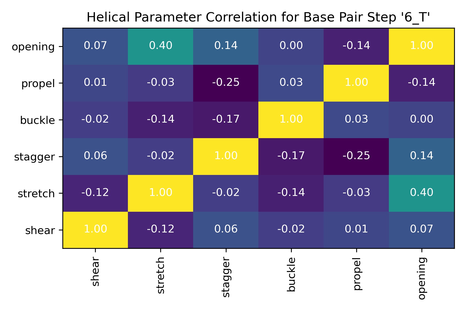
Helical Parameter Correlations: Intra-base pair

from biobb_dna.intrabp_correlations.intrahpcorr import intrahpcorr

timeseries_shear = timeseries_dir+"/series_shear_"+timesel.value[:-1]+".csv"
timeseries_stretch = timeseries_dir+"/series_stretch_"+timesel.value[:-1]+".csv"
timeseries_stagger = timeseries_dir+"/series_stagger_"+timesel.value[:-1]+".csv"
timeseries_buckle = timeseries_dir+"/series_buckle_"+timesel.value[:-1]+".csv"
timeseries_propel = timeseries_dir+"/series_propel_"+timesel.value[:-1]+".csv"
timeseries_opening = timeseries_dir+"/series_opening_"+timesel.value[:-1]+".csv"

output_helpar_bp_correlation_csv_path = "helpar_bp_correlation.csv"
output_helpar_bp_correlation_jpg_path = "helpar_bp_correlation.jpg"

intrahpcorr(
    input_filename_shear=timeseries_shear,
    input_filename_stretch=timeseries_stretch,
    input_filename_stagger=timeseries_stagger,
    input_filename_buckle=timeseries_buckle,
    input_filename_propel=timeseries_propel,
    input_filename_opening=timeseries_opening,
    output_csv_path=output_helpar_bp_correlation_csv_path,
    output_jpg_path=output_helpar_bp_correlation_jpg_path)

df = pd.read_csv(output_helpar_bp_correlation_csv_path)
df

	Unnamed: 0	shear	stretch	stagger	buckle	propel	opening
0	shear	1.000000	-0.122310	0.062783	-0.024045	0.012255	0.066297
1	stretch	-0.122310	1.000000	-0.024948	-0.141840	-0.034225	0.396172
2	stagger	0.062783	-0.024948	1.000000	-0.172773	-0.253086	0.138571
3	buckle	-0.024045	-0.141840	-0.172773	1.000000	0.029668	0.000972
4	propel	0.012255	-0.034225	-0.253086	0.029668	1.000000	-0.138484
5	opening	0.066297	0.396172	0.138571	0.000972	-0.138484	1.000000

Image(filename=output_helpar_bp_correlation_jpg_path,width = 600)

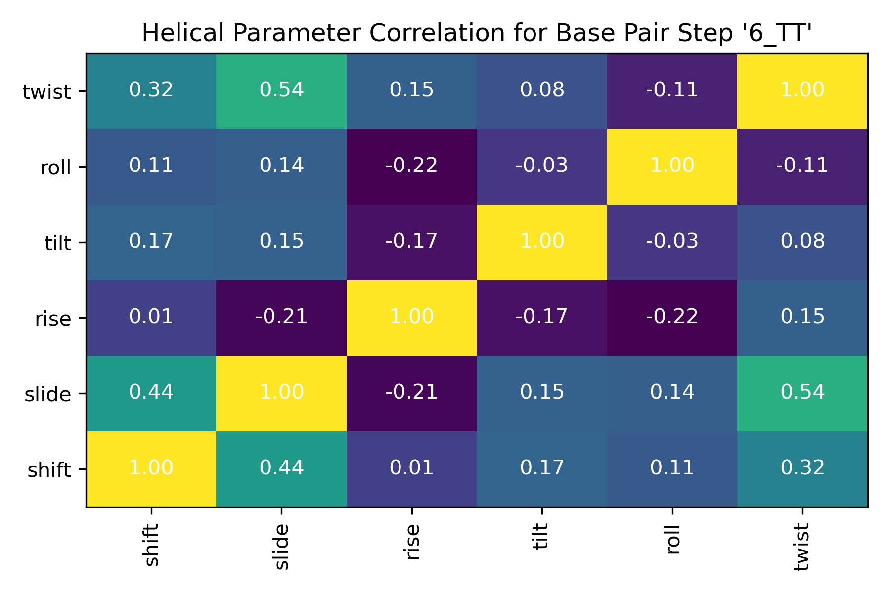
Helical Parameter Correlations: Inter-base pair steps

from biobb_dna.interbp_correlations.interhpcorr import interhpcorr

timeseries_shift = timeseries_dir+"/series_shift_"+timesel.value+".csv"
timeseries_slide = timeseries_dir+"/series_slide_"+timesel.value+".csv"
timeseries_rise = timeseries_dir+"/series_rise_"+timesel.value+".csv"
timeseries_tilt = timeseries_dir+"/series_tilt_"+timesel.value+".csv"
timeseries_roll = timeseries_dir+"/series_roll_"+timesel.value+".csv"
timeseries_twist = timeseries_dir+"/series_twist_"+timesel.value+".csv"

output_helpar_bps_correlation_csv_path = "helpar_bps_correlation.csv"
output_helpar_bps_correlation_jpg_path = "helpar_bps_correlation.jpg"

interhpcorr(
    input_filename_shift=timeseries_shift,
    input_filename_slide=timeseries_slide,
    input_filename_rise=timeseries_rise,
    input_filename_tilt=timeseries_tilt,
    input_filename_roll=timeseries_roll,
    input_filename_twist=timeseries_twist,
    output_csv_path=output_helpar_bps_correlation_csv_path,
    output_jpg_path=output_helpar_bps_correlation_jpg_path)

df = pd.read_csv(output_helpar_bps_correlation_csv_path)
df

	Unnamed: 0	shift	slide	rise	tilt	roll	twist
0	shift	1.000000	0.439831	0.006659	0.166307	0.113906	0.318624
1	slide	0.439831	1.000000	-0.207299	0.151236	0.141627	0.541202
2	rise	0.006659	-0.207299	1.000000	-0.173336	-0.224263	0.147534
3	tilt	0.166307	0.151236	-0.173336	1.000000	-0.032611	0.084610
4	roll	0.113906	0.141627	-0.224263	-0.032611	1.000000	-0.109835
5	twist	0.318624	0.541202	0.147534	0.084610	-0.109835	1.000000

Image(filename=output_helpar_bps_correlation_jpg_path,width = 600)

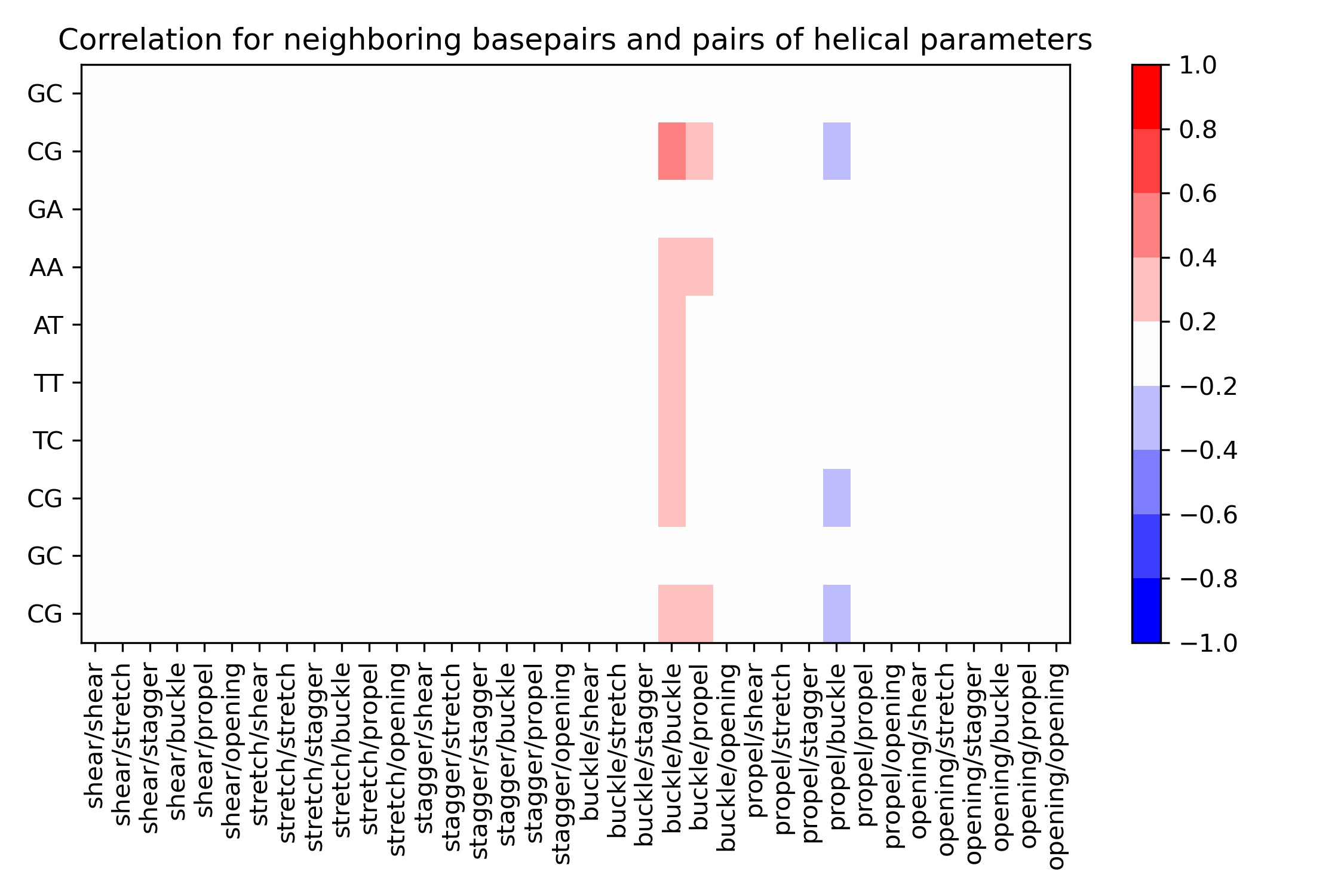
Neighboring steps Correlations: Intra-base pair

from biobb_dna.intrabp_correlations.intrabpcorr import intrabpcorr

canal_shear = canal_dir+"/canal_output_shear.ser"
canal_stretch = canal_dir+"/canal_output_stretch.ser"
canal_stagger = canal_dir+"/canal_output_stagger.ser"
canal_buckle = canal_dir+"/canal_output_buckle.ser"
canal_propel = canal_dir+"/canal_output_propel.ser"
canal_opening = canal_dir+"/canal_output_opening.ser"

output_bp_correlation_csv_path = "bp_correlation.csv"
output_bp_correlation_jpg_path = "bp_correlation.jpg"

prop = {
    'sequence' : seq
}

intrabpcorr(
    input_filename_shear=canal_shear,
    input_filename_stretch=canal_stretch,
    input_filename_stagger=canal_stagger,
    input_filename_buckle=canal_buckle,
    input_filename_propel=canal_propel,
    input_filename_opening=canal_opening,
    output_csv_path=output_bp_correlation_csv_path,
    output_jpg_path=output_bp_correlation_jpg_path,
    properties=prop)

df = pd.read_csv(output_bp_correlation_csv_path)
df

	Unnamed: 0	shear/shear	shear/stretch	shear/stagger	shear/buckle	shear/propel	shear/opening	stretch/shear	stretch/stretch	stretch/stagger	...	propel/stagger	propel/buckle	propel/propel	propel/opening	opening/shear	opening/stretch	opening/stagger	opening/buckle	opening/propel	opening/opening
0	GC	-0.005642	0.018630	-0.025087	-0.010539	0.024243	0.019345	-0.011061	0.021519	-0.020824	...	-0.024222	0.005585	0.006706	-0.021960	-0.010185	0.006839	-0.011742	0.001443	0.005266	0.019129
1	CG	0.020041	0.051434	0.001951	-0.059043	0.027216	0.045336	-0.051213	-0.033895	0.009731	...	0.047045	-0.335039	-0.122872	-0.067494	-0.047289	-0.037659	0.023410	-0.105277	-0.082899	0.005289
2	GA	-0.037801	0.027801	-0.015043	-0.105601	0.073992	0.025790	-0.010322	0.043308	0.011708	...	0.073619	-0.176741	-0.051962	0.003138	0.029520	0.005160	0.051622	0.007026	-0.017732	0.021906
3	AA	0.023788	-0.000117	-0.004595	-0.027747	-0.031901	-0.041804	0.023817	-0.006556	-0.005822	...	-0.061579	-0.147203	-0.004269	-0.050649	-0.039697	0.035455	-0.018540	-0.093678	-0.048917	0.042879
4	AT	0.032575	0.003270	-0.028156	-0.070385	-0.066959	0.021602	0.014530	0.014772	-0.047132	...	-0.113304	-0.173226	0.107649	0.019869	-0.036929	-0.020634	-0.030510	0.021788	0.036952	0.119437
5	TT	-0.010285	-0.009504	0.035414	0.004137	0.003110	0.052842	-0.020711	0.005863	-0.007229	...	-0.091332	-0.132041	0.183310	0.023056	-0.051025	0.023035	-0.017409	0.003068	0.010977	0.191239
6	TC	0.002390	0.003433	-0.024093	0.014480	-0.012981	0.059420	0.030606	0.011428	0.005235	...	-0.019650	-0.152708	0.080905	0.021846	-0.012044	0.067861	-0.083172	0.048029	0.028434	0.151051
7	CG	-0.027842	0.002501	0.014905	0.010619	0.018963	0.030263	-0.020690	0.016758	0.033150	...	0.063238	-0.222382	0.012536	-0.021479	-0.042303	0.020077	0.014984	-0.018558	-0.076957	0.006822
8	GC	-0.030918	0.025377	0.047997	-0.149693	0.032799	0.004369	-0.029652	0.018781	0.037963	...	0.063868	-0.188492	-0.044925	-0.027264	-0.025809	0.027768	0.030092	-0.062296	0.025229	0.019334
9	CG	-0.001727	0.039837	0.013472	-0.031293	-0.014562	0.043469	-0.018693	-0.008573	0.026310	...	0.044891	-0.303367	-0.113362	-0.080200	-0.018591	-0.029267	0.032287	-0.095808	-0.074735	-0.005167

10 rows × 37 columns

Image(filename=output_bp_correlation_jpg_path,width = 800)

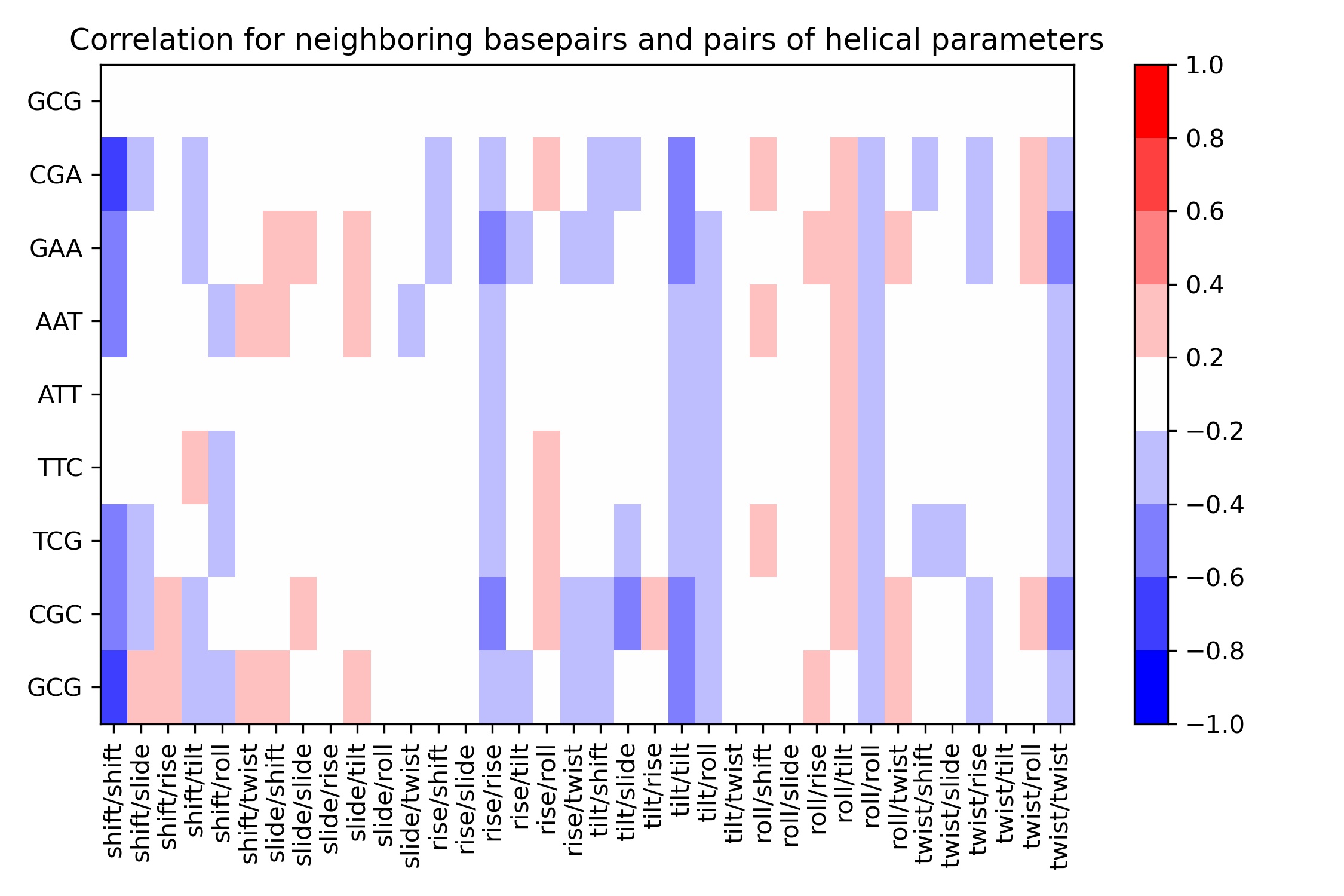
Neighboring steps Correlations: Inter-base pair steps

from biobb_dna.interbp_correlations.interbpcorr import interbpcorr

canal_shift = canal_dir+"/canal_output_shift.ser"
canal_slide = canal_dir+"/canal_output_slide.ser"
canal_rise = canal_dir+"/canal_output_rise.ser"
canal_tilt = canal_dir+"/canal_output_tilt.ser"
canal_roll = canal_dir+"/canal_output_roll.ser"
canal_twist = canal_dir+"/canal_output_twist.ser"

output_bps_correlation_csv_path = "bps_correlation.csv"
output_bps_correlation_jpg_path = "bps_correlation.jpg"

prop = {
    'sequence' : seq
}

interbpcorr(
    input_filename_shift=canal_shift,
    input_filename_slide=canal_slide,
    input_filename_rise=canal_rise,
    input_filename_tilt=canal_tilt,
    input_filename_roll=canal_roll,
    input_filename_twist=canal_twist,
    output_csv_path=output_bps_correlation_csv_path,
    output_jpg_path=output_bps_correlation_jpg_path,
    properties=prop)

df = pd.read_csv(output_bps_correlation_csv_path)
df

	Unnamed: 0	shift/shift	shift/slide	shift/rise	shift/tilt	shift/roll	shift/twist	slide/shift	slide/slide	slide/rise	...	roll/rise	roll/tilt	roll/roll	roll/twist	twist/shift	twist/slide	twist/rise	twist/tilt	twist/roll	twist/twist
0	GCG	-0.034515	-0.013978	0.028504	-0.016774	0.007526	-0.019706	-0.005945	0.003258	0.016998	...	-0.024289	0.034074	-0.014922	0.002918	0.024087	0.011902	-0.018600	-0.000658	0.004749	0.031633
1	CGA	-0.620729	-0.213534	0.153552	-0.379811	-0.069482	0.090324	-0.185796	0.035204	-0.072609	...	0.185182	0.239957	-0.327237	0.146238	-0.301986	-0.066687	-0.230273	-0.149935	0.234940	-0.358276
2	GAA	-0.556258	-0.055634	0.106571	-0.307558	-0.124963	0.111320	0.336513	0.207062	0.010327	...	0.243220	0.222142	-0.356105	0.262547	-0.112359	-0.169531	-0.267369	-0.017553	0.222109	-0.448559
3	AAT	-0.422776	0.121578	0.172917	-0.120018	-0.234489	0.333776	0.200294	0.055308	-0.062561	...	0.182963	0.269344	-0.261031	0.037170	-0.055827	-0.035366	-0.125160	-0.008524	0.080896	-0.336058
4	ATT	-0.135159	0.048764	0.052558	0.152407	-0.137398	0.093877	-0.058611	0.177430	0.140074	...	0.189502	0.241552	-0.262516	0.016017	-0.027548	-0.024130	-0.059852	-0.003261	0.031997	-0.293106
5	TTC	-0.115228	0.074008	0.011805	0.204128	-0.216200	-0.032101	-0.028032	0.184504	0.114301	...	0.113645	0.247625	-0.299766	-0.015864	-0.148998	0.111239	0.075143	0.053240	-0.015885	-0.273020
6	TCG	-0.428290	-0.230813	0.116441	0.057122	-0.208447	-0.118440	-0.121029	0.055468	0.090725	...	0.093449	0.287541	-0.273905	0.101453	-0.316904	-0.253028	-0.076103	-0.114819	0.066582	-0.335519
7	CGC	-0.577276	-0.389311	0.286179	-0.324285	-0.179625	0.071846	0.054698	0.233093	-0.148480	...	0.140274	0.210203	-0.362062	0.244422	-0.150061	-0.097582	-0.265051	-0.021533	0.240612	-0.447802
8	GCG	-0.626682	0.229957	0.290226	-0.338901	-0.240202	0.328321	0.213949	0.040634	0.007077	...	0.287660	0.196857	-0.327687	0.263437	-0.127565	-0.149207	-0.200700	-0.092674	0.171328	-0.372676

9 rows × 37 columns

Image(filename=output_bps_correlation_jpg_path,width = 800)

---

Questions & Comments

Questions, issues, suggestions and comments are really welcome!

• GitHub issues:

  • https://github.com/bioexcel/biobb

• BioExcel forum:

  • https://ask.bioexcel.eu/c/BioExcel-Building-Blocks-library